Boosting as a Species Distribution Model in R

Author

Elke Windschitl

Published

December 2, 2022

Introduction

In this post, I attempt to reproduce work by Elith et al. 2008¹ to model species distribution of short-finned eel (Anguilla australis) using Boosted Regression Trees. This analysis was created for an assignment for EDS 232 Machine Learning in Environmental Science – a course in UCSB’s Master’s of Environmental Data Science curriculum taught by Mateo Robbins.

Boosting is a popular machine learning algorithm that builds models sequentially based on information learned from the previous model². Here, decision trees will be built in sequence using extreme gradient boosting to classify presence or absence of short-finned eel in a given location associated with environmental parameters such as temperature, slope, rainy days, etc. Elith et al. used package gbm in R, whereas I use a Tidymodels approach in R.

Data

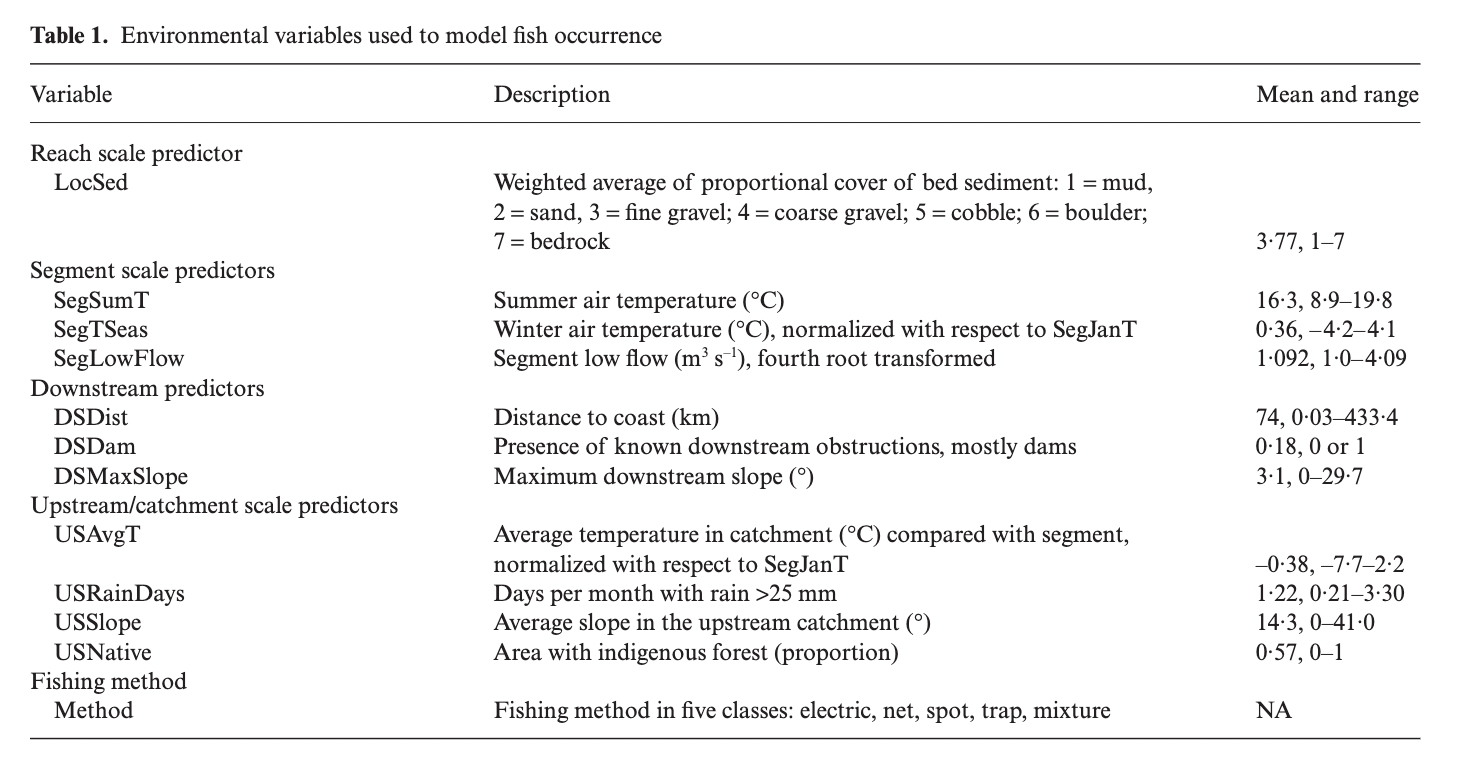
Data labeled “model.data.csv” were retrieved from the supplemental information by Elith et al. 2008 and include the following variables:

Figure 1: Table 1. from Elith et al. 2008 displaying the variables included in the analysis.

# Load libraries
library(tidyverse)
library(tidymodels)
library(sjPlot)
library(pROC)
library(RColorBrewer)
library(knitr)

eel_data <- eel_data_raw %>%
  select(-Site) # remove site number from data frame
eel_data$Angaus <- as.factor(eel_data$Angaus) # set outcome variable as a factor

eel_data %>% slice_head(n = 5) %>% kable

Angaus	SegSumT	SegTSeas	SegLowFlow	DSDist	DSMaxSlope	USAvgT	USRainDays	USSlope	USNative	DSDam	Method	LocSed
0	16.0	-0.10	1.036	50.20	0.57	0.09	2.470	9.8	0.81	0	electric	4.8
1	18.7	1.51	1.003	132.53	1.15	0.20	1.153	8.3	0.34	0	electric	2.0
0	18.3	0.37	1.001	107.44	0.57	0.49	0.847	0.4	0.00	0	spo	1.0
0	16.7	-3.80	1.000	166.82	1.72	0.90	0.210	0.4	0.22	1	electric	4.0
1	17.2	0.33	1.005	3.95	1.15	-1.20	1.980	21.9	0.96	0	electric	4.7

Methods

Split and Resample

I split the data from above into a training and test set 70/30, stratified by outcome score. I used 10-fold CV to resample the training set, stratified by Angaus.

# Stratified sampling with the rsample package
set.seed(123) # Set a seed for reproducibility
split <- initial_split(data = eel_data, 
                       prop = .7, 
                       strata = "Angaus")

eel_train <- training(split) # Grab training data
eel_test  <- testing(split) # Grab test data

# Set up cross validation stratified on Angaus
cv_folds <- eel_train %>% 
  vfold_cv(v=10, strata = "Angaus")

Preprocessing

I created a recipe to prepare the data for the XGBoost model. I was interested in predicting the binary outcome variable Angaus which indicates presence or absence of the eel species Anguilla australis.

# Set up a recipe
eel_rec <- recipe(Angaus ~ ., data = eel_train) %>% 
  step_dummy(all_nominal(), -all_outcomes(), one_hot = TRUE) %>% 
  prep(training = eel_train, retain = TRUE)

# Bake to check recipe
baked_eel <- bake(eel_rec, eel_train)

Tuning XGBoost

Tune Learning Rate

First I conducted tuning on just the learn_rate parameter.

eel_spec <- parsnip::boost_tree(mode = "classification",
                                engine = "xgboost",
                                trees = 1000,
                                learn_rate = tune())

I set up a grid to tune my model by using a range of learning rate parameter values.

# Set up tuning grid
eel_grid <- expand.grid(learn_rate = seq(0.0001, 0.5, length.out = 50))

# Set up workflow
wf_eel_tune <- workflow() %>% 
  add_recipe(eel_rec) %>% 
  add_model(eel_spec)

doParallel::registerDoParallel(cores = 3)
set.seed(123)

# Tune
eel_rs <- tune_grid(
  wf_eel_tune,
  Angaus~.,
  resamples = cv_folds,
  grid = eel_grid
)

# Identify best values from the tuning process
eel_rs %>%
  tune::show_best(metric = "accuracy") %>%
  slice_head(n = 5) %>% 
  kable(caption = "Performance of the best models and the associated estimates for the learning rate parameter values.")

Performance of the best models and the associated estimates for the learning rate parameter values.
learn_rate	.metric	.estimator	mean	n	std_err	.config
0.0205041	accuracy	binary	0.8327667	10	0.0108841	Preprocessor1_Model03
0.2041408	accuracy	binary	0.8327248	10	0.0115023	Preprocessor1_Model21
0.3367673	accuracy	binary	0.8312542	10	0.0095568	Preprocessor1_Model34
0.2755551	accuracy	binary	0.8312347	10	0.0096176	Preprocessor1_Model28
0.0103020	accuracy	binary	0.8298475	10	0.0094675	Preprocessor1_Model02

  # tab_df(title = "Table 2",
  #        digits = 4,
  #        footnote = "Performance of the best models and the associated estimates for the learning rate parameter values.",
  #        show.footnote = TRUE)

eel_best_learn <- eel_rs %>%
  tune::select_best("accuracy")

# eel_model <- eel_spec %>% 
#   finalize_model(eel_best_learn)

Tune Tree Parameters

I created a new specification where I set the learning rate and tune the tree parameters.

eel_spec2 <- parsnip::boost_tree(mode = "classification",
                                engine = "xgboost",
                                trees = 1000,
                                learn_rate = eel_best_learn$learn_rate,
                                min_n = tune(),
                                tree_depth = tune(),
                                loss_reduction = tune()
                                )

I set up a tuning grid using grid_max_entropy() to get a representative sampling of the parameter space.

# Define parameters to be tuned
eel_params <- dials::parameters(
  min_n(),
  tree_depth(),
  loss_reduction()
)

# Set up grid
eel_grid2 <- dials::grid_max_entropy(eel_params, size = 50)

# Set up workflow
wf_eel_tune2 <- workflow() %>% 
  add_recipe(eel_rec) %>% 
  add_model(eel_spec2)

set.seed(123)
doParallel::registerDoParallel(cores = 3)

# Tune
eel_rs2 <- tune_grid(
  wf_eel_tune2,
  Angaus~.,
  resamples = cv_folds,
  grid = eel_grid2
)

# Identify best values from the tuning process
eel_rs2 %>%
  tune::show_best(metric = "accuracy") %>% 
  slice_head(n = 5) %>% 
  kable(caption = "Performance of the best models and the associated estimates for the tree parameter values.")

Performance of the best models and the associated estimates for the tree parameter values.
min_n	tree_depth	loss_reduction	.metric	.estimator	mean	n	std_err	.config
5	10	0.0045022	accuracy	binary	0.8499315	10	0.0143809	Preprocessor1_Model35
10	4	0.0001488	accuracy	binary	0.8455026	10	0.0114082	Preprocessor1_Model18
5	13	1.4059617	accuracy	binary	0.8441143	10	0.0116907	Preprocessor1_Model11
6	12	0.0000219	accuracy	binary	0.8385017	10	0.0136802	Preprocessor1_Model14
12	14	0.0000002	accuracy	binary	0.8369507	10	0.0106411	Preprocessor1_Model22

  # tab_df(title = "Table 3",
  #        digits = 4,
  #        footnote = "Performance of the best models and the associated estimates for the tree parameter values.",
  #        show.footnote = TRUE)

eel_best_trees <- eel_rs2 %>%
  tune::select_best("accuracy")

# eel_model2 <- eel_spec2 %>% 
#   finalize_model(eel_best_trees)

Tune Stochastic Parameters

I created another new specification where I set the learning rate and tree parameters and tune the stochastic parameters.

eel_spec3 <- parsnip::boost_tree(mode = "classification",
                                engine = "xgboost",
                                trees = 1000,
                                learn_rate = eel_best_learn$learn_rate,
                                min_n = eel_best_trees$min_n,
                                tree_depth = eel_best_trees$tree_depth,
                                mtry = tune(),                   
                                loss_reduction = eel_best_trees$loss_reduction,
                                sample_size = tune(),
                                stop_iter = tune()
                                )

I set up a tuning grid using grid_max_entropy() again.

# Define parameters to be tuned
eel_params2 <- dials::parameters(
  finalize(mtry(),select(baked_eel,-Angaus)),
  sample_size = sample_prop(c(.4, .9)),
  stop_iter())

# Set up grid
eel_grid3 <- dials::grid_max_entropy(eel_params2, size = 50)

# Set up workflow
wf_eel_tune3 <- workflow() %>% 
  add_recipe(eel_rec) %>% 
  add_model(eel_spec3)

set.seed(123)
doParallel::registerDoParallel(cores = 3)

# Tune
eel_rs3 <- tune_grid(
  wf_eel_tune3,
  Angaus~.,
  resamples = cv_folds,
  grid = eel_grid3
)

# Identify best values from the tuning process
eel_rs3 %>%
  tune::show_best(metric = "accuracy") %>%
  slice_head(n = 5) %>% 
  kable(caption = "Performance of the best models and the associated estimates for the stochastic parameter values.")

Performance of the best models and the associated estimates for the stochastic parameter values.
mtry	sample_size	stop_iter	.metric	.estimator	mean	n	std_err	.config
9	0.6101083	17	accuracy	binary	0.8398688	10	0.0095528	Preprocessor1_Model42
7	0.6760456	11	accuracy	binary	0.8398285	10	0.0101101	Preprocessor1_Model29
14	0.4702631	19	accuracy	binary	0.8384603	10	0.0104765	Preprocessor1_Model44
4	0.4148151	3	accuracy	binary	0.8384597	10	0.0112940	Preprocessor1_Model04
11	0.8900167	14	accuracy	binary	0.8384402	10	0.0103511	Preprocessor1_Model16

  # tab_df(title = "Table 4",
  #        digits = 4,
  #        footnote = "Performance of the best models and the associated estimates for the stochastic parameter values.",
  #        show.footnote = TRUE)

eel_best_stoch <- eel_rs3 %>%
  tune::select_best("accuracy")

eel_model3 <- eel_spec3 %>% 
  finalize_model(eel_best_stoch)

Finalize workflow

I assembled my final workflow with all of my optimized parameters and did a final fit.

eel_final_spec <- parsnip::boost_tree(mode = "classification",
                                engine = "xgboost",
                                trees = 1000,
                                learn_rate = eel_best_learn$learn_rate,
                                min_n = eel_best_trees$min_n,
                                tree_depth = eel_best_trees$tree_depth,
                                mtry = eel_best_stoch$mtry,                   
                                loss_reduction = eel_best_trees$loss_reduction,
                                stop_iter = eel_best_stoch$stop_iter,
                                sample_size = eel_best_stoch$sample_size
                                )

# Set up workflow
wf_eel_final <- workflow() %>% 
  add_recipe(eel_rec) %>% 
  add_model(eel_final_spec)

final_simple_fit <- wf_eel_final %>% # fit to just training data (need for later)
  fit(data = eel_train)

final_eel_fit <- last_fit(eel_final_spec, Angaus~., split) # does training fit then final prediction as well

# Show predictions
final_pred_tab <- as.data.frame(final_eel_fit$.predictions)
head(final_pred_tab) %>% 
  kable(caption = "Predictions of Angaus presence on test data.")

Predictions of Angaus presence on test data.
.pred_0	.pred_1	.row	.pred_class	Angaus	.config
0.9937342	0.0062658	1	0	0	Preprocessor1_Model1
0.1122560	0.8877440	2	1	1	Preprocessor1_Model1
0.7499388	0.2500612	3	0	0	Preprocessor1_Model1
0.6484206	0.3515794	4	0	0	Preprocessor1_Model1
0.9473680	0.0526320	9	0	0	Preprocessor1_Model1
0.4369654	0.5630346	10	1	1	Preprocessor1_Model1

final_met_tab <- final_eel_fit$.metrics # Store metrics
head(final_met_tab) %>% 
  kable(caption = "Accuracy and area under ther receiver operator curve of the final fit.")

Accuracy and area under ther receiver operator curve of the final fit.

.metric	.estimator	.estimate	.config
accuracy	binary	0.8305648	Preprocessor1_Model1
roc_auc	binary	0.8209016	Preprocessor1_Model1

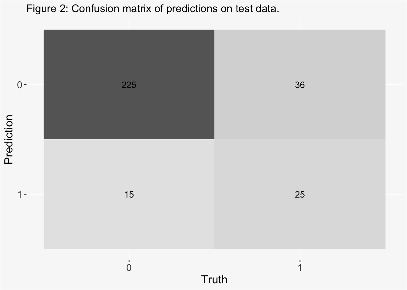
# Bind predictions and original data
eel_test_rs <- cbind(eel_test, final_eel_fit$.predictions)
eel_test_rs <- eel_test_rs[,-1] # Remove duplicate column

# Compute a confusion matrix
cm<- eel_test_rs %>% yardstick::conf_mat(truth = Angaus, estimate = .pred_class) 

autoplot(cm, type = "heatmap") +
  theme(axis.text.x = element_text(size = 12),
        axis.text.y = element_text(size = 12),
        axis.title = element_text(size = 14),
        panel.background = element_rect(fill = "#F8F8F8"),
        plot.background = element_rect(fill = "#F8F8F8")) +
  labs(title = "Figure 2: Confusion matrix of predictions on test data.")

tibble <- final_eel_fit %>% collect_metrics()

final_eel_accuracy <- tibble %>%
  filter(.metric == "accuracy") %>%
  pull(.estimate)

final_eel_auc <- tibble %>%
  filter(.metric == "roc_auc") %>%
  pull(.estimate)

The model had an accuracy of 0.83. The ROC area under the curve was 0.82. The rate of false negatives was 0.12, and the rate of false positives was 0.05.

The model had an accuracy of 0.83. The ROC area under the curve was 0.82. The rate of false negatives was 0.12, and the rate of false positives was 0.05.

Results

I then fit my final model to the evaluation data set labeled “eel.eval.data.csv” and compare performances.

# Read in eval data
eval_dat <- eval_dat_raw %>% 
  rename(Angaus = Angaus_obs) %>% # rename to match previous data
  mutate(Angaus = as_factor(Angaus)) # make outcome a factor

prediction <- final_simple_fit %>% predict(new_data = eval_dat) # generate predictions
eval_dat_pred <- cbind(eval_dat, prediction)

# Compare predicted classes to actual classes
correct_predictions <- sum(eval_dat_pred$.pred_class == eval_dat_pred$Angaus)

# Calculate accuracy
accuracy <- correct_predictions / nrow(eval_dat_pred)

# Calculate auc
eval_dat_pred$pred_num <- as.numeric(eval_dat_pred$.pred_class)
auc <- auc(eval_dat_pred$Angaus, eval_dat_pred$pred_num)

How did my model perform on this data?

The model had an accuracy of 0.832on these data, which isn’t quite as good as the accuracy when applying the model to the testing data. However the difference is not too extreme and seems pretty good given that the dummy classifier would be 0.744. The model had an AUC of 0.7 which is not great.

How did my results compare to those of Elith et al.?

The model here does not do as well as the model in Elith et al. which found a model AUC of 0.858. My AUC of 0.7 is disappointingly far off. This could be because the data have imbalanced classes. Elith et al. did more tuning to find the optimal values and used larger ranges of trees, where as I was more limited by computing power on my laptop. They also could have tuned the threshold for classification, which I did not do here. I also used a Tidymodels approach, where as it is possible that the gbm package offers more power or flexibility when tuning.

References

¹Elith, J., Leathwick, J.R. and Hastie, T. (2008), A working guide to boosted regression trees. Journal of Animal Ecology, 77: 802-813. https://doi.org/10.1111/j.1365-2656.2008.01390.x

²Boehmke, Bradley, and Brandon Greenwell. “Chapter 12 Gradient Boosting.” Hands-On Machine Learning with R, 2020, https://bradleyboehmke.github.io/HOML/gbm.html. Accessed 3 Oct. 2023.