# Import necessary packages
import ee
import geemap
import numpy as np
import pandas as pd
import matplotlib.pyplot as plt
import ipyleaflet

# Authenticate and initialize Google Earth Engine
#ee.Authenticate()
ee.Initialize()Exploring Changes in Iowa’s Cropland with Google Earth Engine and Python
Description: Here I use Python to access the Google Earth Engine API and explore how Iowa’s cropland has changed between 2003 and 2022.
Introduction:
Iowa is an agriculture state. It is a major hub for corn and soy. In fact, my great-grandparents used to farm Iowa land. So how has Iowa’s cropland changed over time? Here I begin exploring that question using remote sensing products accessed through Google Earth Engine.
The Data:
I use the Cropland Data Layer created by the USDA, National Agricultural Statistics Service (NASS), Research and Development Division, Geospatial Information Branch, Spatial Analysis Research Section1. This dataset has been reported annually since 1997, but 2003 is the first year where coverage accross Iowa is complete. I use 2003 and 2022 in my explorations. I also use the FAO GAUL: Global Administrative Unit Layers 2015, First-Level Administrative Units to clip the cropland data to the state of Iowa2.
Methods & Results:
I start by importing all necessary libraries/modules and reading in all data. I use ee for accessing the Google Earth Engine data, and geemap for mapping the rasters. NumpPy and Pandas are for handling tabular data. Matplotlib is used to visualize results.
I read in the administrative boundary data and filter for the US and Iowa.
# Read in boundary gee data
boundaries = ee.FeatureCollection("FAO/GAUL/2015/level1")
# Apply the filter to get Iowa
iowa = boundaries.filter(ee.Filter.eq("ADM0_NAME", "United States of America")) \
    .filter(ee.Filter.eq("ADM1_NAME", "Iowa"))
I read in the crop data, filter for my years of interest and clip to the state of iowa.
# Read in crop data from gee
crop_dat = ee.ImageCollection("USDA/NASS/CDL")
crop_vis = {'bands': ['cropland']}
# Read in crop data from GEE for the year 2003
cropland_03 = crop_dat \
.filterDate('2003') \
.first() \
.clip(iowa)
# Read in crop data from GEE for the year 2022
cropland_22 = crop_dat \
.filterDate('2022') \
.first() \
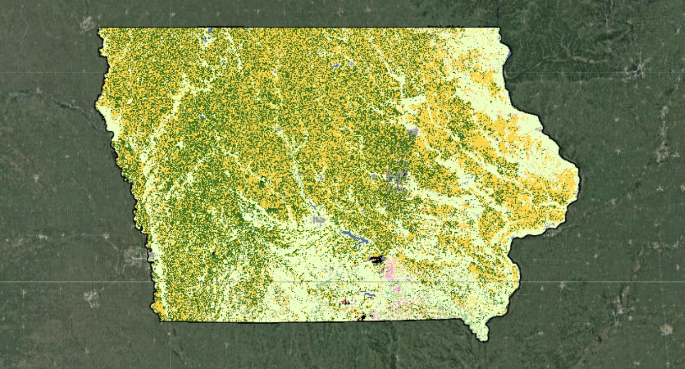
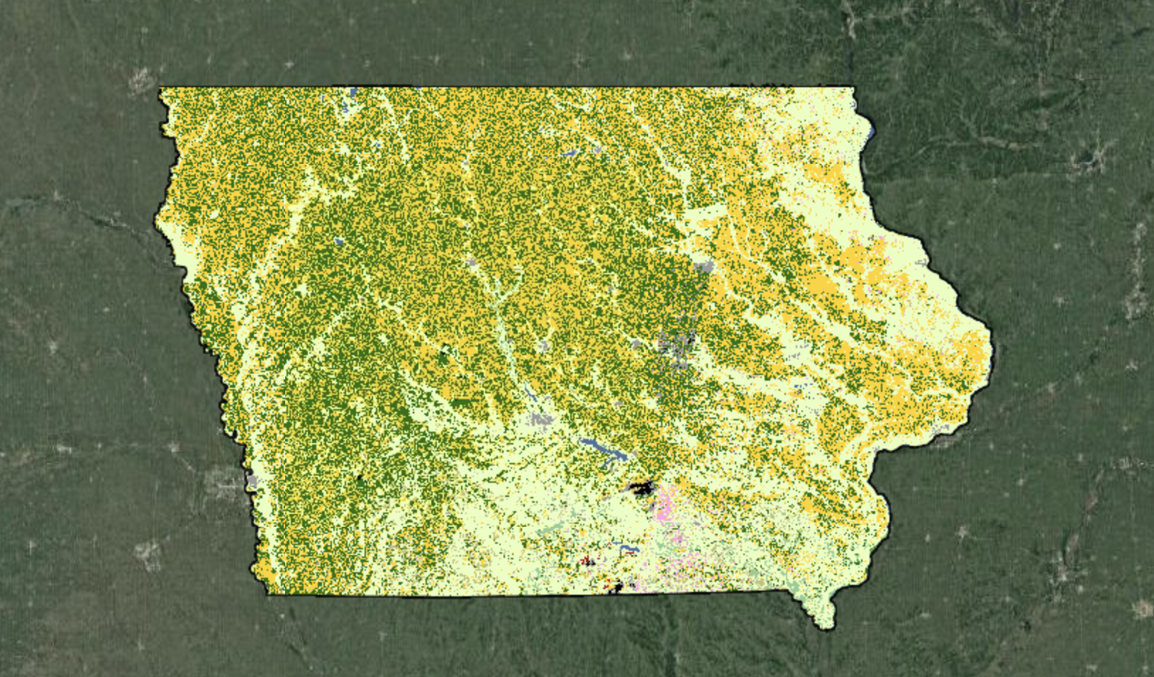
.clip(iowa)Let’s explore the cropland use in Iowa in 2003.
# Create a map
Map_03 = geemap.Map()

# Change basemap
Map_03.add_basemap('SATELLITE')

# Add iowa and center/zoom
Map_03.addLayer(iowa)
Map_03.centerObject(iowa, 6)

# Add your raster data to the map
Map_03.addLayer(cropland_03, crop_vis, 'Landcover')
Map_03.add_legend(title="USDA Land and Crop Classification", builtin_legend='USDA/NASS/CDL')

# Display the map
display(Map_03)
Note
Quarto does not seem to consistently render GEE maps. This is something I am still trouble-shooting. Because of this, I have included pictures of the outputs, and a link to the Jupyter Notebook.
Let’s explore the cropland use in Iowa in 2022.
# Create a map
Map_22 = geemap.Map()

# Change basemap
Map_22.add_basemap('SATELLITE')

# Add iowa and center/zoom
Map_22.addLayer(iowa)
Map_22.centerObject(iowa, 6)

# Add your raster data to the map
Map_22.addLayer(cropland_22, crop_vis, 'Landcover')
Map_22.add_legend(title="USDA Land and Crop Classification", builtin_legend='USDA/NASS/CDL')

# Display the map
display(Map_22)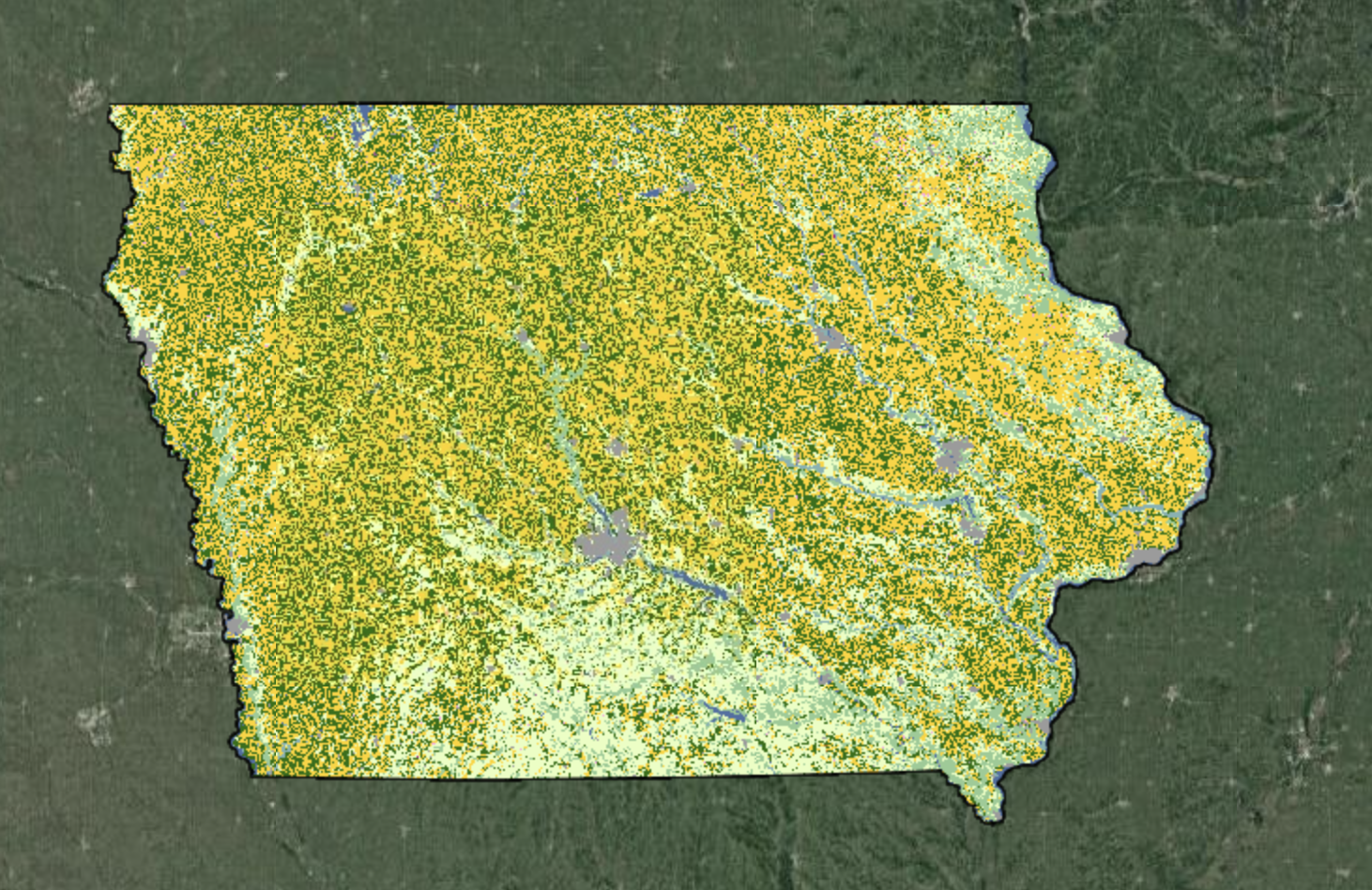
I used the image_area_by_group function from geepmap to calculate the area of each type of crop in each year. Now I have tabular data I can work with as well.
# Reduce for image_area_by_group to work properly
reduced_03 = crop_dat.select('cropland').filterDate('2003').reduce(ee.Reducer.mode()).clip(iowa)
reduced_22 = crop_dat.select('cropland').filterDate('2022').reduce(ee.Reducer.mode()).clip(iowa)
# Calculate square km of each group for each year and create dataframe
areas_03 = geemap.image_area_by_group(reduced_03, scale=1000, denominator=1e6,decimal_places=4, verbose=False)
areas_22 = geemap.image_area_by_group(reduced_22, scale=1000, denominator=1e6,decimal_places=4, verbose=False)
I also create a dataframe of the specified legend colors designated by the USDA.
Code
# Create dictionary of colors so we can use them in vis later (I don't think I can extract from built-in colors)
legend_dict = {
    '1 Corn': '#ffd300',
    '2 Cotton': '#ff2626',
    '3 Rice': '#00a8e2',
    '4 Sorghum': '#ff9e0a',
    '5 Soybeans': '#267000',
    '6 Sunflower': '#ffff00',
    '10 Peanuts': '#70a500',
    '11 Tobacco': '#00af49',
    '12 Sweet Corn': '#dda50a',
    '13 Pop or Orn Corn': '#dda50a',
    '14 Mint': '#7cd3ff',
    '21 Barley': '#e2007c',
    '22 Durum Wheat': '#896054',
    '23 Spring Wheat': '#d8b56b',
    '24 Winter Wheat': '#a57000',
    '25 Other Small Grains': '#d69ebc',
    '26 Dbl Crop WinWht/Soybeans': '#707000',
    '27 Rye': '#aa007c',
    '28 Oats': '#a05989',
    '29 Millet': '#700049',
    '30 Speltz': '#d69ebc',
    '31 Canola': '#d1ff00',
    '32 Flaxseed': '#7c99ff',
    '33 Safflower': '#d6d600',
    '34 Rape Seed': '#d1ff00',
    '35 Mustard': '#00af49',
    '36 Alfalfa': '#ffa5e2',
    '37 Other Hay/Non Alfalfa': '#a5f28c',
    '38 Camelina': '#00af49',
    '39 Buckwheat': '#d69ebc',
    '41 Sugarbeets': '#a800e2',
    '42 Dry Beans': '#a50000',
    '43 Potatoes': '#702600',
    '44 Other Crops': '#00af49',
    '45 Sugarcane': '#af7cff',
    '46 Sweet Potatoes': '#702600',
    '47 Misc Vegs & Fruits': '#ff6666',
    '48 Watermelons': '#ff6666',
    '49 Onions': '#ffcc66',
    '50 Cucumbers': '#ff6666',
    '51 Chick Peas': '#00af49',
    '52 Lentils': '#00ddaf',
    '53 Peas': '#54ff00',
    '54 Tomatoes': '#f2a377',
    '55 Caneberries': '#ff6666',
    '56 Hops': '#00af49',
    '57 Herbs': '#7cd3ff',
    '58 Clover/Wildflowers': '#e8bfff',
    '59 Sod/Grass Seed': '#afffdd',
    '60 Switchgrass': '#00af49',
    '61 Fallow/Idle Cropland': '#bfbf77',
    '63 Forest': '#93cc93',
    '64 Shrubland': '#c6d69e',
    '65 Barren': '#ccbfa3',
    '66 Cherries': '#ff00ff',
    '67 Peaches': '#ff8eaa',
    '68 Apples': '#ba004f',
    '69 Grapes': '#704489',
    '70 Christmas Trees': '#007777',
    '71 Other Tree Crops': '#af9970',
    '72 Citrus': '#ffff7c',
    '74 Pecans': '#b5705b',
    '75 Almonds': '#00a582',
    '76 Walnuts': '#e8d6af',
    '77 Pears': '#af9970',
    '81 Clouds/No Data': '#f2f2f2',
    '82 Developed': '#999999',
    '83 Water': '#4970a3',
    '87 Wetlands': '#7cafaf',
    '88 Nonag/Undefined': '#e8ffbf',
    '92 Aquaculture': '#00ffff',
    '111 Open Water': '#4970a3',
    '112 Perennial Ice/Snow': '#d3e2f9',
    '121 Developed/Open Space': '#999999',
    '122 Developed/Low Intensity': '#999999',
    '123 Developed/Med Intensity': '#999999',
    '124 Developed/High Intensity': '#999999',
    '131 Barren': '#ccbfa3',
    '141 Deciduous Forest': '#93cc93',
    '142 Evergreen Forest': '#93cc93',
    '143 Mixed Forest': '#93cc93',
    '152 Shrubland': '#c6d69e',
    '176 Grassland/Pasture': '#e8ffbf',
    '190 Woody Wetlands': '#7cafaf',
    '195 Herbaceous Wetlands': '#7cafaf',
    '204 Pistachios': '#00ff8c',
    '205 Triticale': '#d69ebc',
    '206 Carrots': '#ff6666',
    '207 Asparagus': '#ff6666',
    '208 Garlic': '#ff6666',
    '209 Cantaloupes': '#ff6666',
    '210 Prunes': '#ff8eaa',
    '211 Olives': '#334933',
    '212 Oranges': '#e27026',
    '213 Honeydew Melons': '#ff6666',
    '214 Broccoli': '#ff6666',
    '215 Avocados': '#739755',
    '216 Peppers': '#ff6666',
    '217 Pomegranates': '#af9970',
    '218 Nectarines': '#ff8eaa',
    '219 Greens': '#ff6666',
    '220 Plums': '#ff8eaa',
    '221 Strawberries': '#ff6666',
    '222 Squash': '#ff6666',
    '223 Apricots': '#ff8eaa',
    '224 Vetch': '#00af49',
    '225 Dbl Crop WinWht/Corn': '#ffd300',
    '226 Dbl Crop Oats/Corn': '#ffd300',
    '227 Lettuce': '#ff6666',
    '228 Dbl Crop Triticale/Corn': '#f8d248',
    '229 Pumpkins': '#ff6666',
    '230 Dbl Crop Lettuce/Durum Wht': '#896054',
    '231 Dbl Crop Lettuce/Cantaloupe': '#ff6666',
    '232 Dbl Crop Lettuce/Cotton': '#ff2626',
    '233 Dbl Crop Lettuce/Barley': '#e2007c',
    '234 Dbl Crop Durum Wht/Sorghum': '#ff9e0a',
    '235 Dbl Crop Barley/Sorghum': '#ff9e0a',
    '236 Dbl Crop WinWht/Sorghum': '#a57000',
    '237 Dbl Crop Barley/Corn': '#ffd300',
    '238 Dbl Crop WinWht/Cotton': '#a57000',
    '239 Dbl Crop Soybeans/Cotton': '#267000',
    '240 Dbl Crop Soybeans/Oats': '#267000',
    '241 Dbl Crop Corn/Soybeans': '#ffd300',
    '242 Blueberries': '#000099',
    '243 Cabbage': '#ff6666',
    '244 Cauliflower': '#ff6666',
    '245 Celery': '#ff6666',
    '246 Radishes': '#ff6666',
    '247 Turnips': '#ff6666',
    '248 Eggplants': '#ff6666',
    '249 Gourds': '#ff6666',
    '250 Cranberries': '#ff6666',
    '254 Dbl Crop Barley/Soybeans': '#267000'
}

# Create a DataFrame from the legend dictionary
legend_df = pd.DataFrame(list(legend_dict.items()), columns=['num_crop', 'color'])
legend_df['crop'] = legend_df['num_crop'].apply(lambda x: x.split(' ', 1)[1])
legend_df['group'] = legend_df['num_crop'].apply(lambda x: x.split(' ', 1)[0])
legend_df| num_crop | color | crop | group | |
|---|---|---|---|---|
| 0 | 1 Corn | #ffd300 | Corn | 1 |
| 1 | 2 Cotton | #ff2626 | Cotton | 2 |
| 2 | 3 Rice | #00a8e2 | Rice | 3 |
| 3 | 4 Sorghum | #ff9e0a | Sorghum | 4 |
| 4 | 5 Soybeans | #267000 | Soybeans | 5 |
| ... | ... | ... | ... | ... |
| 128 | 247 Turnips | #ff6666 | Turnips | 247 |
| 129 | 248 Eggplants | #ff6666 | Eggplants | 248 |
| 130 | 249 Gourds | #ff6666 | Gourds | 249 |
| 131 | 250 Cranberries | #ff6666 | Cranberries | 250 |
| 132 | 254 Dbl Crop Barley/Soybeans | #267000 | Dbl Crop Barley/Soybeans | 254 |
133 rows × 4 columns
I join the color data to the area data for consistent color use when plotting.
# Reset the index of the areas DataFrame
areas_03.reset_index(inplace=True)

# Merge the existing DataFrame with the legend DataFrame based on the 'group' column & sort
crop_areas_03 = pd.merge(areas_03, legend_df, on='group', how='left')
crop_areas_03['year'] = 2003
area_sorted_03 = crop_areas_03.sort_values(by='area', ascending=False)

# Reset the index of the areas DataFrame
areas_22.reset_index(inplace=True)

# Merge the existing DataFrame with the legend DataFrame based on the 'group' column & sort
crop_areas_22 = pd.merge(areas_22, legend_df, on='group', how='left')
crop_areas_22['year'] = 2022
area_sorted_22 = crop_areas_22.sort_values(by='area', ascending=False)
Let’s check out the top 10 crops each year by area
area_sorted_03.head(10)| group | area | percentage | num_crop | color | crop | year | |
|---|---|---|---|---|---|---|---|
| 0 | 1 | 52415.6902 | 0.3599 | 1 Corn | #ffd300 | Corn | 2003 |
| 13 | 176 | 42853.8696 | 0.2942 | 176 Grassland/Pasture | #e8ffbf | Grassland/Pasture | 2003 |
| 1 | 5 | 41927.8154 | 0.2879 | 5 Soybeans | #267000 | Soybeans | 2003 |
| 7 | 61 | 2933.1871 | 0.0201 | 61 Fallow/Idle Cropland | #bfbf77 | Fallow/Idle Cropland | 2003 |
| 8 | 63 | 1673.6551 | 0.0115 | 63 Forest | #93cc93 | Forest | 2003 |
| 4 | 36 | 1472.0163 | 0.0101 | 36 Alfalfa | #ffa5e2 | Alfalfa | 2003 |
| 10 | 82 | 1370.3573 | 0.0094 | 82 Developed | #999999 | Developed | 2003 |
| 11 | 83 | 478.8680 | 0.0033 | 83 Water | #4970a3 | Water | 2003 |
| 2 | 25 | 218.6646 | 0.0015 | 25 Other Small Grains | #d69ebc | Other Small Grains | 2003 |
| 9 | 81 | 186.8087 | 0.0013 | 81 Clouds/No Data | #f2f2f2 | Clouds/No Data | 2003 |
area_sorted_22.head(10)| group | area | percentage | num_crop | color | crop | year | |
|---|---|---|---|---|---|---|---|
| 0 | 1 | 57108.8402 | 0.3918 | 1 Corn | #ffd300 | Corn | 2022 |
| 1 | 5 | 43917.2096 | 0.3013 | 5 Soybeans | #267000 | Soybeans | 2022 |
| 25 | 176 | 25775.1745 | 0.1769 | 176 Grassland/Pasture | #e8ffbf | Grassland/Pasture | 2022 |
| 22 | 141 | 10638.4229 | 0.0730 | 141 Deciduous Forest | #93cc93 | Deciduous Forest | 2022 |
| 18 | 122 | 1590.3012 | 0.0109 | 122 Developed/Low Intensity | #999999 | Developed/Low Intensity | 2022 |
| 26 | 190 | 1503.0166 | 0.0103 | 190 Woody Wetlands | #7cafaf | Woody Wetlands | 2022 |
| 16 | 111 | 1291.7266 | 0.0089 | 111 Open Water | #4970a3 | Open Water | 2022 |
| 17 | 121 | 999.4524 | 0.0069 | 121 Developed/Open Space | #999999 | Developed/Open Space | 2022 |
| 19 | 123 | 901.4150 | 0.0062 | 123 Developed/Med Intensity | #999999 | Developed/Med Intensity | 2022 |
| 27 | 195 | 759.0405 | 0.0052 | 195 Herbaceous Wetlands | #7cafaf | Herbaceous Wetlands | 2022 |
Let’s plot corn, soybean, and grassland/pasture to see how their area’s have changed over the 20 years.
# Create a grouped bar plot
plt.figure(figsize=(9, 6))

# Define colors
lightgray = '#f5f5f5'
darkgray = '#2b2b2b'

# Define crops/landcover of interest
selected_crops = ['Corn', 'Soybeans', 'Grassland/Pasture']

# Set bar choices
bar_width = 0.4
bar_positions_2003 = np.arange(len(selected_crops))
bar_positions_2022 = bar_positions_2003 + bar_width + 0.05

# Plot bars for 2003
for i, crop in enumerate(selected_crops):
    crop_data_2003 = area_sorted_03[(area_sorted_03['crop'] == crop) & (area_sorted_03['year'] == 2003)]
    plt.bar(bar_positions_2003[i], crop_data_2003['area'].values[0], width=bar_width, color=crop_data_2003['color'].values[0], label=crop)

# Plot bars for 2022
for i, crop in enumerate(selected_crops):
    crop_data_2022 = area_sorted_22[(area_sorted_22['crop'] == crop) & (area_sorted_22['year'] == 2022)]
    plt.bar(bar_positions_2022[i], crop_data_2022['area'].values[0], width=bar_width, color=crop_data_2022['color'].values[0])

# Set background color
plt.gca().set_facecolor(darkgray)
fig = plt.gcf()
fig.patch.set_facecolor(darkgray)

# Set labels and their aesthetics
plt.xlabel('Year', fontname='Arial', color=lightgray, size = 12)
plt.ylabel('Area (km$^2$)', fontname='Arial', color=lightgray, size = 12)
plt.title('Area of Selected Landcover in 2003 and 2022 by Type', fontname='Arial', color=lightgray, size=16)

# Adjust x-axis ticks to include both years
plt.xticks(np.concatenate([bar_positions_2003, bar_positions_2022]), [2003, 2003, 2003, 2022, 2022, 2022], fontname='Arial', color=lightgray)
plt.yticks(color=lightgray)

# Set border color
plt.gca().spines['bottom'].set_color(lightgray)
plt.gca().spines['top'].set_color(lightgray)
plt.gca().spines['right'].set_color(lightgray)
plt.gca().spines['left'].set_color(lightgray)

# Set tick marks color
plt.tick_params(axis='both', colors='lightgray')

# Set legend text color
legend = plt.legend(title='Crop/Type', bbox_to_anchor=(.72, .97), loc='upper left', prop={'family': 'Arial'})
plt.setp(legend.get_title(), color=darkgray)
for text in legend.get_texts():
    text.set_color(darkgray)

plt.show()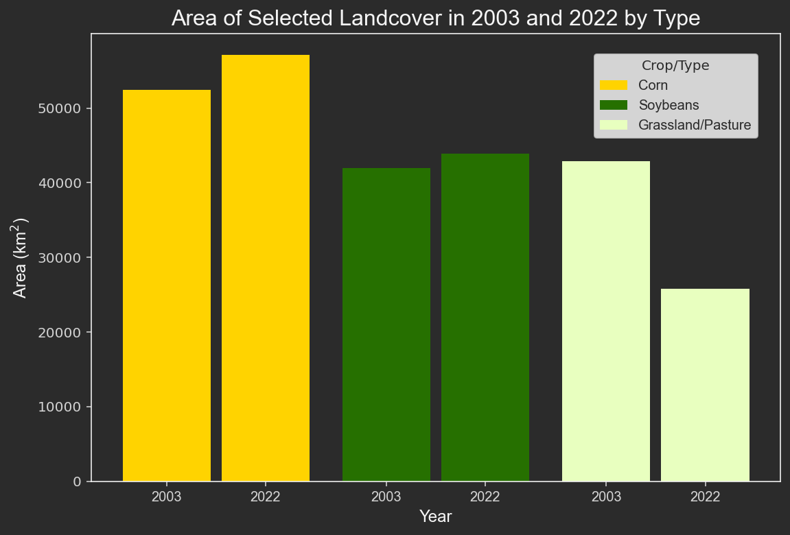
Conclusions
Unsurprisingly, Iowa’s land cover has changed a bit over the years, but corn remains the predominant crop. Google Earth Engine allowed me to smoothly access, use, and visualize a remote sensing data product. Further analyses could be completed to identify changes in crops through all years or what landcover type has had the largest % change over time.
References:
1USDA National Agricultural Statistics Service Cropland Data Layer. 2022. Published crop-specific data layer [Online]. Available at https://nassgeodata.gmu.edu/CropScape/ (accessed 12/03/2023). USDA-NASS, Washington, DC.
2FAO GAUL: Global Administrative Unit Layers 2015, First-Level Administrative Units. 2015. Available at https://developers.google.com/earth-engine/datasets/catalog/FAO_GAUL_2015_level1#terms-of-use (accessed 12/03/2023). FAO UN, Rome, Italy.