# Load libraries
library(sf)
library(terra)
library(readr)
library(raster)
library(dplyr)
library(ggplot2)
library(maptiles)
library(tidyterra)
library(ggspatial)
library(cowplot)

#---- Set up the data directory
#data_dir <- insert your file path to your dataMapping Locations for Kelp Aquaculture in R
Description: In this qmd, I create a publishable map of locations that have habitat that is likely suitable for kelp aquaculture near Santa Barbara.
Introduction
While earning my master’s of environmental data science from the University of California, Santa Barbara, I completed a group capstone project with three other peers. Our clients included Natalie Dornan, a researcher at UCSB, and Ocean Rainforest, an aquaculture company with operations in Santa Barbara. We were tasked with combining open source data sets on giant kelp and various oceanographic factors in the region to create one synthesized data product. We were asked to use that data product to model habitat suitability for giant kelp to aid Ocean Rainforest in siting aquaculture projects in the future. Here, I map the final results of those efforts.
The Data
I used six types of data in this process. I used the model results from our species distribution habitat suitability modeling, kelp data, substrate data, and boundary data of state boundaries, federal boundaries, and marine protected areas. Metadata on these data sources can be found in the kelpGeoMod data repository.
Methods
First I load all of the libraries I will need. I use sf for handling shapefiles and vector data. I use terra and raster for handling raster data. readr is used to read in data, and dplyr is used for any data frame manipulation. I use ggplot to make my plots, but I leverage maptiles to get basemaps and tidyterra to use the basemap with ggplot. ggspatial is used to place a scale and arrow on the maps, and cowplot is used to plot maps together.
I read in all of the necessary datasets from my local machine.
# Read in data
# Read in project AOI
aoi <- st_read(file.path(data_dir, "02-intermediate-data/02-aoi-sbchannel-shapes-intermediate/aoi-sbchannel.shp"))

# Read in federal boundaries
fed_bounds <- st_read(file.path(data_dir, "01-raw-data/federal_boundaries/USMaritimeLimitsNBoundaries.shp")) %>%
  filter(REGION == "Pacific Coast")

# Read in the 3-nautical mile state boundary
state_bounds <- st_read(file.path(data_dir, "01-raw-data/state_boundaries/stanford-sg211gq3741-shapefile/sg211gq3741.shp"))

# Read in MPAs
mpas <- st_read(file.path(data_dir, "01-raw-data/04-mpa-boundaries-raw/California_Marine_Protected_Areas_[ds582]/California_Marine_Protected_Areas_[ds582].shp"))

# Read in sandy-bottom raster
sandy_raster <- raster(file.path(data_dir, "03-analysis-data/05-substrate-analysis/sandy-bottom-1km.tif"))

# Read in kelp brick
kelp <- brick(file.path(data_dir, "02-intermediate-data/05-kelp-area-biomass-intermediate/kelp-area-brick.tif"))

# Read in the maxent modeling outputs
maxent_quarter_1 <- raster(file.path(data_dir, "03-analysis-data/04-maxent-analysis/results/maxent-quarter-1-output.tif"))
maxent_quarter_2 <- raster(file.path(data_dir, "03-analysis-data/04-maxent-analysis/results/maxent-quarter-2-output.tif"))
maxent_quarter_3 <- raster(file.path(data_dir, "03-analysis-data/04-maxent-analysis/results/maxent-quarter-3-output.tif"))
maxent_quarter_4 <- raster(file.path(data_dir, "03-analysis-data/04-maxent-analysis/results/maxent-quarter-4-output.tif"))
For the mapping, I want to find locations from the model output where raster grid cells…
Have a minimum of 0.4 habitat suitability in ALL quarters
Did not have any kelp seen in them (as of 2014-2022 from remotely sensed data)
Have sandy-bottom substrate
Because our client wouldn’t want to place an aquaculture effort where kelp already exists, we need to define where kelp has been seen growing in the past 6 years. My teammate, Erika, perfomed analyses to find the average amount of kelp in each grid cell by season. Here is that code:
# (Code from Erika)
# Create function to average kelp area per grid cell over all years by quarter
calc_seasonal_means_brick <- function(rast_to_convert) {

  quarter_sets <- list(seq(from = 1, to = 36, by = 4), # Q1s (winter)
                       seq(from = 2, to = 36, by = 4), # Q2s (spring)
                       seq(from = 3, to = 36, by = 4), # Q3s (summer)
                       seq(from = 4, to = 36, by = 4)) # Q4s (fall)

  all_seasons_brick <- brick() # set up brick to hold averaged layers for each season (will have 4 layers at the end)

  for (i in seq_along(quarter_sets)) {

    season_brick_holder <- brick() # hold all layers for one season, then reset for next season

    for (j in quarter_sets[[i]]) {
      season_brick <- brick() # hold single layer in a season, then reset for next layer
      season_brick <- addLayer(season_brick, rast_to_convert[[j]]) # add single layer to initialized brick
      season_brick_holder <- addLayer(season_brick_holder, season_brick) # add this layer to the holder for this season, and repeat until have all layers from season
    }

    season_averaged_layer <- calc(season_brick_holder, mean) # after having all layers from season, take the mean
    all_seasons_brick <- addLayer(all_seasons_brick, season_averaged_layer) # add mean to the brick holding all averaged layers, and then repeat for the next season
  }

  return(all_seasons_brick) # return the resulting brick object
}

kelp_all <- calc_seasonal_means_brick(rast_to_convert = kelp)

kelp_quarter1 <- kelp_all[[1]]
kelp_quarter2 <- kelp_all[[2]]
kelp_quarter3 <- kelp_all[[3]]
kelp_quarter4 <- kelp_all[[4]]
Masking the model output
As you can see from the quick plot below, the model output shows where along the Santa Barbara coastline has the highest predicted habitat suitability for kelp in each quarter. However, that information alone is not necessarily helpful in citing a new aquaculture farm.
# quick plot maxent output
plot(maxent_quarter_1)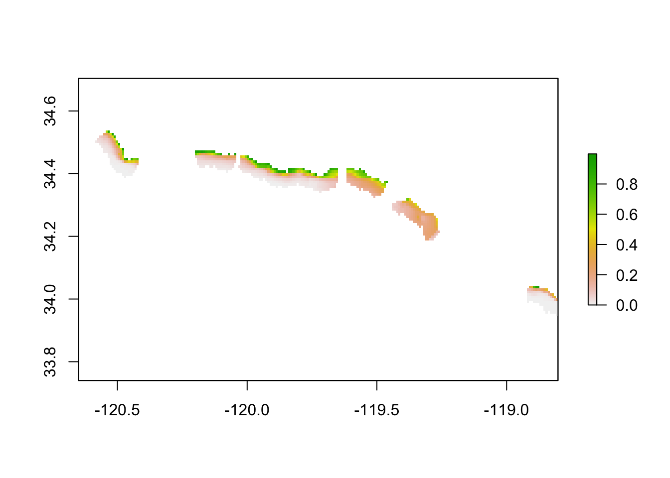
Also, you might note that there are gaps in the output. Unfortunately available data did not cover the entire Santa Barbara Channel. Our results are therefore limited.
To find locations that match our clients’ needs, we need to do some further analysis and masking. First, I reclassify areas that have less than 40% likelihood of habitability to NA to remove them from our raster output. I do this for each quarter. I also mask out areas where kelp has already been seen growing. I stack and mask the quarters in a way that cells where there is existing kelp or a <0.4 probability of suitability in ANY of the quarters gets removed from the raster. Then I create one raster with the mean probability of suitability for elegible locations thus far. Here is that process and the resulting raster.
# Prep data
# Reclassify values <0.4 to NA for each quarter and mask out areas with kelp
rcl_1 <- maxent_quarter_1 %>%
  reclassify(cbind(0, 0.4, NA), right=FALSE) %>%
  mask(mask = kelp_quarter1, inverse = TRUE)
rcl_2 <- maxent_quarter_2 %>%
  reclassify(cbind(0, 0.4, NA), right=FALSE) %>%
  mask(mask = kelp_quarter2, inverse = TRUE)
rcl_3 <- maxent_quarter_3 %>%
 reclassify(cbind(0, 0.4, NA), right=FALSE) %>%
  mask(mask = kelp_quarter3, inverse = TRUE)
rcl_4 <- maxent_quarter_4 %>%
 reclassify(cbind(0, 0.4, NA), right=FALSE) %>%
  mask(mask = kelp_quarter4, inverse = TRUE)

good_cells_stack <- stack(rcl_1, rcl_2, rcl_3, rcl_4) #stack

# Mask to areas that meet a minimum of 0.4 for all quarters
# Create an empty raster with the same extent and resolution as the input rasters
maxent_mask <- raster(good_cells_stack[[1]])
values(maxent_mask) <- 1  # Set all cells in the mask raster to a common value

# Iterate over each raster and update the mask raster where they overlap
for (i in 1:4) {
  maxent_mask <- maxent_mask * (good_cells_stack[[i]])  # Update the mask where raster values are zero
}

# Mask rcl_1
masked_rcl_1 <- mask(rcl_1, maxent_mask)
# Mask rcl_2
masked_rcl_2 <- mask(rcl_2, maxent_mask)
# Mask rcl_3
masked_rcl_3 <- mask(rcl_3, maxent_mask)
# Mask rcl_4
masked_rcl_4 <- mask(rcl_4, maxent_mask)


# Take the mean value of all four quarters
mean_masked_maxent <- mean(masked_rcl_1, masked_rcl_2, masked_rcl_3, masked_rcl_4)
plot(mean_masked_maxent)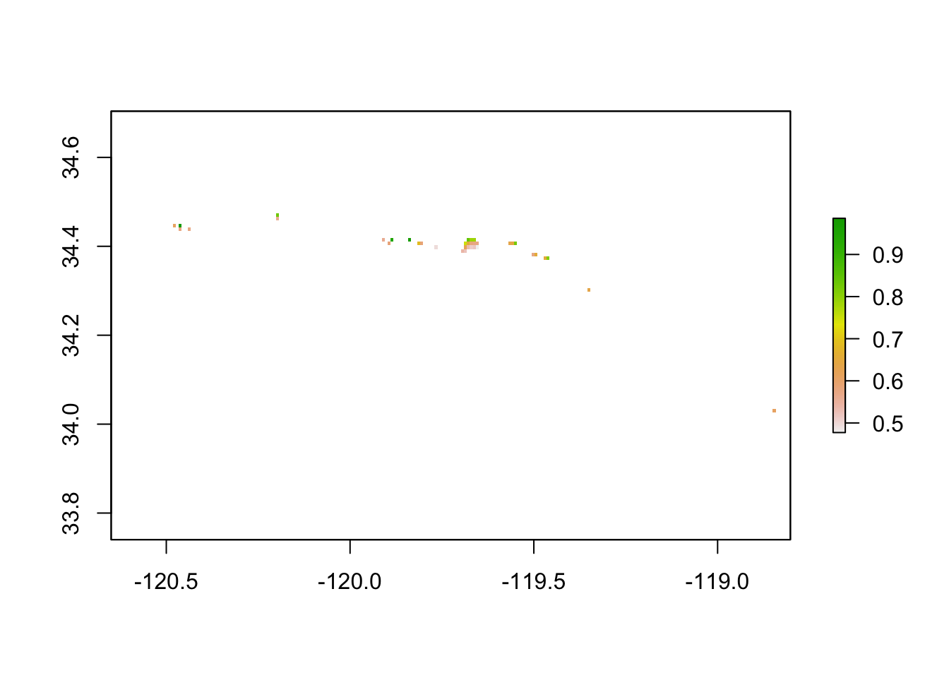
I’m most of the way there! Rocky-bottom seafloor is important habitat, so our client needs sandy-bottom seafloor to place aquaculture infrastructure and start a kelp farm. I only keep raster grid cells where sandy-bottom seafloor is present.
# Convert to package terra
sandy_terra <- rast(sandy_raster)
maxent_terra <- rast(mean_masked_maxent)

# Mask maxent to areas with sandy-bottom
sub_masked_model <- terra::mask(x = maxent_terra, mask = sandy_terra, inverse = FALSE)
Next, I prepare the other layers of my map. I ensure that their coordinate reference system matches my habitat layer, and I intersect to retrieve shapes only in the area of interest (plus a slight buffer).
# Transform to get every layer in same crs
aoi <- st_transform(aoi, crs = 4326)
mpas <- st_transform(mpas, crs = 4326)
fed_bounds <- st_transform(fed_bounds, crs = 4326)
state_bounds <- st_transform(state_bounds, crs = 4326)

# Define the amount of aoi buffer I want
buffer_size <- 10000

# Create a buffer around the AOI
buffered_aoi <- st_buffer(aoi, buffer_size)

# Reduce shape file data sets to only in my area of interest + buffer
aoi_mpas <- st_intersection(mpas, buffered_aoi)
aoi_fed_bounds <- st_intersection(fed_bounds, buffered_aoi)
aoi_state_bounds <- st_intersection(state_bounds, buffered_aoi)
I use the MPA layer to remove locations from the habitat map within any Marine Protected Area. In this case, there was only one suitable location within an MPA. I then convert to point data for better mapping.
# Remove na values from raster
no_na <- mask(sub_masked_model, !is.na(sub_masked_model))

# Mask out locations within mpas
no_na_no_mpa <- mask(no_na, aoi_mpas, inverse = TRUE)

# Convert to point data
target_points <- as.data.frame(no_na_no_mpa, xy = TRUE, na.rm = TRUE) %>%
  st_as_sf(coords = c("x", "y"),
           crs = st_crs(4326))
I map my results using ggplot with a baselayer, state boundaries, federal boundaries, and marine protected areas. I create two maps – one showing the entire area of interest, and one zoomed in to where the suitable habitat is located. I also make a custom legend to showcase what various boundaries in the map represent. Below I show each of these individual pieces.
# Dowload tiles and compose raster (SpatRaster)
basemap <- get_tiles(
  x = buffered_aoi, provider = "CartoDB.DarkMatterNoLabels", crop = TRUE,
  cachedir = tempdir(), verbose = TRUE
)

# Get smaller box for inset map bounds
small_box <- tribble(
  ~lat, ~lon,
  34.35, -119.54412,
  34.5, -120.30751,
  34.35, -120.30751,
  34.5, -119.54412
) |>
  st_as_sf(coords = c("lon", "lat"),
           crs = "EPSG: 4326") |>
  st_bbox() |>
  st_as_sfc()

# Plot the full AOI
big_plot <- ggplot() +
  geom_spatraster_rgb(
  mapping = aes(),
  basemap,
  interpolate = TRUE,
  r = 1,
  g = 2,
  b = 3
) +
  geom_sf(data = aoi_fed_bounds,
          linetype = "dotdash") +

  geom_sf(data = aoi_state_bounds,
          col = "black",
          alpha = 0,
          linetype = "solid",
          linewidth = 0.3) +

  geom_sf(data = aoi_mpas,
          fill = "#a6a6a6",
          colour = "#a6a6a6",
          alpha = 0.1) +

  geom_sf(data = aoi,
          color = "#203e63",
          alpha = 0,
          linewidth = 0.8) +

  geom_sf(data = target_points,
          color = "#849638",
          size = 0.05) +

  geom_sf(data = small_box,
          colour = "#de8728",
          alpha = 0,
          linewidth = 0.1) +
  theme(panel.background = element_blank(),
        plot.background = element_blank(),
        axis.ticks = element_blank(),
        axis.text = element_blank(),
        panel.grid = element_blank()) +
  annotation_scale(pad_x = unit(1.1, "in"),
                   pad_y = unit(0.55, "in"),
                   bar_cols = c("black", "#262626"),
                   height = unit(0.25, "cm"),
                   text_col = "#a6a6a6") +
  annotation_north_arrow(pad_x = unit(0.6, "in"),
                         pad_y = unit(0.45, "in"),
                         height = unit(0.25, "in"),
                         width = unit(0.3, "in"),
                         style = north_arrow_orienteering(fill = c("black", "#262626"),
                                                          text_col = "#a6a6a6"))

big_plot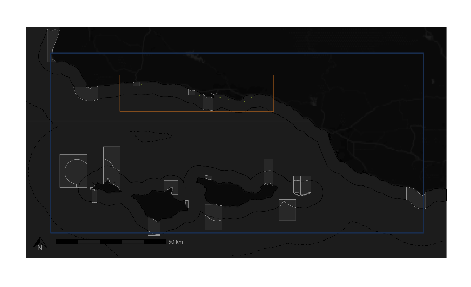
# Create a custom legend plot
legend_plot <- ggplot() +
  geom_segment(aes(x = 0, xend = 1, y = 0, yend = 0, linetype = "1"), color = "black", linewidth = 2) +
  geom_segment(aes(x = 0, xend = 1, y = -1, yend = -1, linetype = "2"), color = "black", linewidth = 2) +
  geom_segment(aes(x = 0, xend = 1, y = -2, yend = -2, linetype = "3"), color = "#a6a6a6", linewidth = 2) +
  geom_segment(aes(x = 0, xend = 1, y = -3, yend = -3, linetype = "4"), color = "#203e63", linewidth = 2) +
  scale_linetype_manual(values = c("solid", "dotdash", "solid", "solid")) +
  theme(panel.background = element_blank(),
        plot.background = element_blank(),
        axis.ticks = element_blank(),
        axis.text = element_blank(),
        axis.title = element_blank(),
        panel.grid = element_blank(),
        panel.margin = margin(c(0,0,500,0)),
        plot.margin = margin(c(0,0,10,0))) +
  coord_cartesian(clip = "off") +
    theme(legend.position = "none") +
  annotate("text",
           x = .33,
           y = -.3,
           label = "State Boundary",
           color = "black",
           size = 12)+
  annotate("text",
           x = .38,
           y = -1.3,
           label = "Federal Boundary",
           color = "black",
           size = 12)+
  annotate("text",
           x = .47,
           y = -2.3,
           label = "Marine Protected Area",
           color = "#a6a6a6",
           size = 12) +
  annotate("text",
           x = .39,
           y = -3.3,
           label = "Project Study Area",
           color = "#203e63",
           size = 12)

legend_plot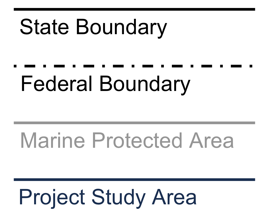
# Save the legend using this trick:
# In RStudio, click on "Zoom", and then zoom the plot to the size and aspect ratio that satisfy you;
# Right click on the plot, then "Copy Image Address", paste the address somewhere, you get the width (www) and height (hhh) information in the address;
# ggsave("plot.png", width = www/90, height = hhh/90, dpi = 900) ggsave("plot.pdf", width = www/90, height = hhh/90)
#https://stackoverflow.com/questions/75020376/save-plot-exactly-as-previewed-in-the-plots-panel
# http://127.0.0.1:35585/graphics/plot_zoom_png?width=520&height=400
ggsave("images/kelp_legend.png", plot = legend_plot, width = 502/90, height = 400/90, units = "in", dpi = 900)
# Crop mpas and state bounds to the inset map
aoi_mpas2 <- st_crop(mpas, small_box)
aoi_state_bounds2 <- st_crop(state_bounds, small_box)
# Dowload tiles and compose raster (SpatRaster)
basemap2 <- get_tiles(
x = small_box, provider = "CartoDB.DarkMatterNoLabels", crop = TRUE,
cachedir = tempdir(), verbose = TRUE
)
# Plot the inset map
small_plot <- ggplot() +
geom_spatraster_rgb(
mapping = aes(),
basemap2,
interpolate = TRUE,
r = 1,
g = 2,
b = 3
) +
geom_sf(data = aoi_state_bounds2,
col = "black",
alpha = 0,
linetype = "solid",
linewidth = 0.3) +
geom_sf(data = aoi_mpas2,
fill = "#a6a6a6",
colour = "#a6a6a6",
alpha = 0.1) +
geom_sf(data = target_points,
color = "#849638",
size = 2) +
geom_sf(data = small_box,
colour = "#de8728",
alpha = 0,
linewidth = 1) +
annotate("text",
x = -119.6982,
y = 34.43,
label = "Santa Barbara",
color = "#a6a6a6") +
annotate("text",
x = -119.86,
y = 34.43,
label = "Goleta",
color = "#a6a6a6") +
annotate("text",
x = -120.2149,
y = 34.478,
label = "Gaviota",
color = "#a6a6a6") +
theme(panel.background = element_blank(),
plot.background = element_blank(),
axis.ticks = element_blank(),
axis.text = element_blank(),
axis.title = element_blank(),
panel.grid = element_blank()) +
annotation_scale(pad_x = unit(0.7, "in"),
pad_y = unit(0.2, "in"),
bar_cols = c("black", "#262626"),
height = unit(0.25, "cm"),
text_col = "#a6a6a6")
small_plot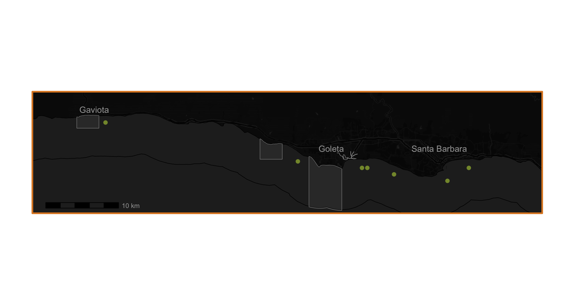
I use cowplot to combine these maps.
# Define the plot background color
bg_color <- "#262626"

# Grab legend from big plot
# legend <- get_legend(big_plot)

# Arrange the plots using plot_grid
combined_plot <- plot_grid(small_plot, big_plot, ncol = 1, axis = "l", rel_heights = c(1, 2.2))

# Set the background color for the entire combined plot + add lines
combined_plot <- combined_plot +
  theme(plot.background = element_blank(),
        axis.ticks = element_blank()) +
    draw_line(
    x = c(0.316, 0.167),
    y = c(0.523, 0.715),
    color = "#de8728", size = 0.2
  ) +
      draw_line(
    x = c(0.56, 0.836),
    y = c(0.523, 0.715),
    color = "#de8728", size = 0.2
  )

# Display the combined plot
print(combined_plot)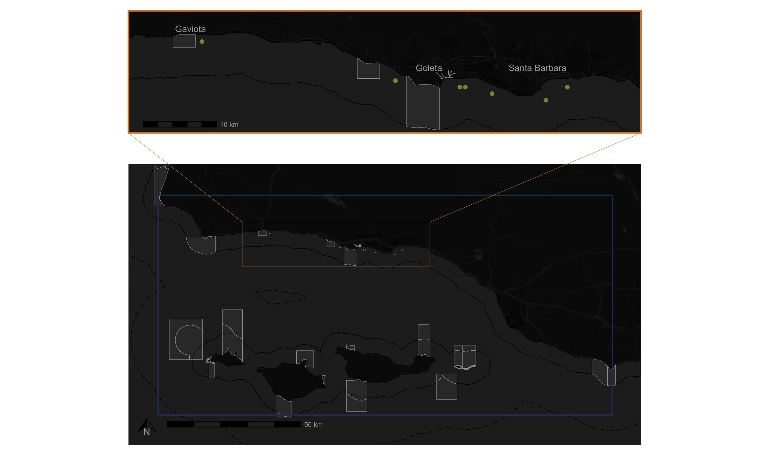
# Save the plot
#http://127.0.0.1:35585/graphics/plot_zoom_png?width=1309&height=796
ggsave("images/kelp_plot.png", plot = combined_plot, width = 1309/90, height = 796/90, units = "in", dpi = 900)
Results
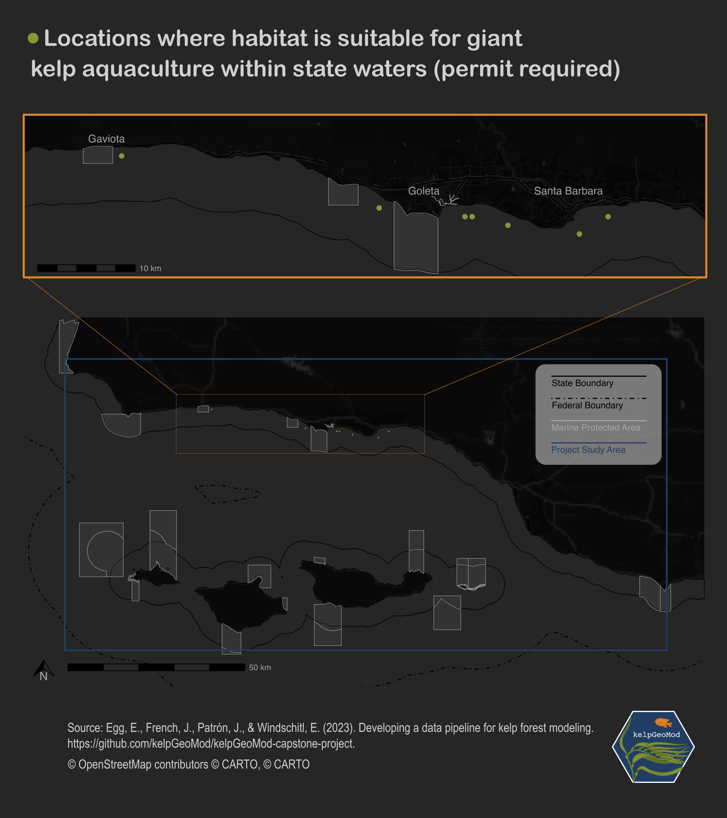
Now that I have the combined map, and a custom legend, I chose to use a graphics editing software to finish off the map. I chose to use Inkscape, which is essentially an open-source version of Adobe Illustrator. In Inkscape I added a title, credits, a background, and our capstone hex logo. Here is the final product!
Please note that these locations are based on habitat suitability – a metric derived from environmental factors. There may be other factors that need to be considered when citing an aquaculture farm that relate to the activities already occurring in those parts of the ocean (such as fishing and boating). Permits must be obtained to conduct aquaculture efforts within state waters. The results of this project are only intended to inform our clients where habitat is most likely suitable for kelp growth.